Particle kinematics is the study of the trajectory of a particle. The position of a particle is defined as the coordinate vector from the origin of a coordinate frame to the particle.

Kinematics of a particle trajectory in a non-rotating frame of reference

In the most general case, a three-dimensional coordinate system is used to define the position of a particle. However, if the particle is constrained to move in a surface, a two-dimensional coordinate system is sufficient. All observations in physics are incomplete without those observations being described with respect to a reference frame.

The position vector of a particle is a vector drawn from the origin of the reference frame to the particle. It expresses both the distance of the point from the origin and its direction from the origin. In three dimensions, the position of point P can be expressed as
where , , and are the Cartesian coordinates and , and are the unit vectors along the , , and coordinate axes, respectively. The magnitude of the position vector gives the distance between the point and the origin.

The direction cosines of the position vector provide a quantitative measure of direction. It is important to note that the position vector of a particle isn’t unique. The position vector of a given particle is different relative to different frames of reference.

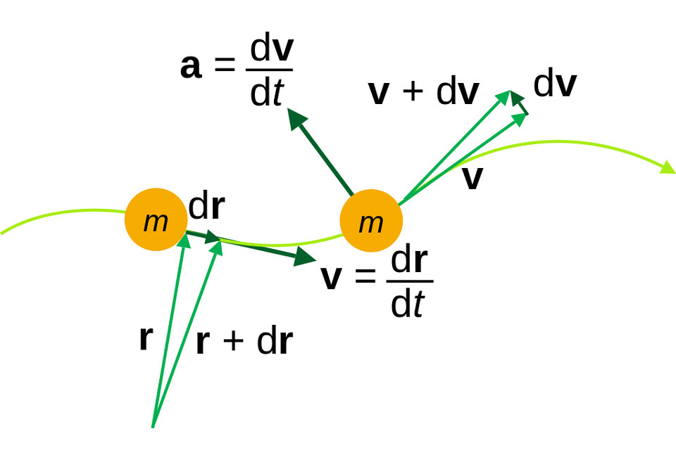
The trajectory of a particle is a vector function of time, , which defines the curve traced by the moving particle, given by

where the coordinates x_P, y_P, and z_P are each functions of time.

Velocity and speed
The velocity of a particle is a vector quantity that describes the direction of motion and the magnitude of the motion of particle. More mathematically, the rate of change of the position vector of a point, with respect to time is the velocity of the point. Consider the ratio formed by dividing the difference of two positions of a particle by the time interval. This ratio is called the average velocity over that time interval and is defined as Velocity=displacement/time taken

where ΔP is the change in the position vector over the time interval Δt.

In the limit as the time interval Δt becomes smaller and smaller, the average velocity becomes the time derivative of the position vector,
The speed of an object is the magnitude |V| of its velocity. It is a scalar quantity:

where s is the arc-length measured along the trajectory of the particle. This arc-length traveled by a particle over time is a non-decreasing quantity. Hence, ds/dt is non-negative, which implies that speed is also non-negative.

Acceleration
The velocity vector can change in magnitude and in direction or both at once. Hence, the acceleration is the rate of change of the magnitude of the velocity vector plus the rate of change of direction of that vector. The same reasoning used with respect to the position of a particle to define velocity, can be applied to the velocity to define acceleration. The acceleration of a particle is the vector defined by the rate of change of the velocity vector. The average acceleration of a particle over a time interval is defined as the ratio.

where ΔV is the difference in the velocity vector and Δt is the time interval.

The acceleration of the particle is the limit of the average acceleration as the time interval approaches zero, which is the time derivative,

or

The magnitude of the acceleration of an object is the magnitude |A| of its acceleration vector. It is a scalar quantity:

Relative position vector

which is the difference between the components of their position vectors.

If point B has position components

then the position of point A relative to point B is the difference between their components:

Relative velocity
The velocity of one point relative to another is simply the difference between their velocities

which is the difference between the components of their velocities.

If point A has velocity components

and point B has velocity components

then the velocity of point A relative to point B is the difference between their components:

Alternatively, this same result could be obtained by computing the time derivative of the relative position vector R_B/A.

In the case where the velocity is close to the speed of light c (generally within 95%), another scheme of relative velocity called rapidity, that depends on the ratio of V to c, is used in special relativity.

Relative acceleration

The acceleration of one point C relative to another point B is simply the difference between their accelerations.

which is the difference between the components of their accelerations.

If point C has acceleration components

and point B has acceleration components

then the acceleration of point C relative to point B is the difference between their components:

Alternatively, this same result could be obtained by computing the second time derivative of the relative position vector P_B/A.

Particle trajectories under constant acceleration
For the case of constant acceleration, the differential equation Eq 1) can be integrated as the acceleration vector A of a point P is constant in magnitude and direction. Such a point is said to undergo uniformly accelerated motion^{. In this case, the velocity V(t) and then the trajectory P(t) of the particle can be obtained by integrating the acceleration equation A with respect to time.}

Assuming that the initial conditions of the position, , and velocity at time are known, the first integration yields the velocity of the particle as a function of time.

A second integration yields its path (trajectory),

Additional relations between displacement, velocity, acceleration, and time can be derived. Since the acceleration is constant, can be substituted into the above equation to give:

A relationship between velocity, position and acceleration without explicit time dependence can be had by solving the average acceleration for time and substituting and simplifying

where ∘ denotes the dot product, which is appropriate as the products are scalars rather than vectors.

The dot can be replaced by the cosine of the angle between the vectors ^{and the vectors by their magnitudes, in which case:}

In the case of acceleration always in the direction of the motion, the angle between the vectors () is 0, so , and

This can be simplified using the notation for the magnitudes of the vectors ^{where can be any curvaceous path taken as the constant tangential acceleration is applied along that path, so}

This reduces the parametric equations of motion of the particle to a cartesian relationship of speed versus position. This relation is useful when time is unknown. We also know that or is the area under a v, t graph. We can take by adding the top area and the bottom area. The bottom area is a rectangle, and the area of a rectangle is the where is the width and is the height. In this case and (note that the here is different from the acceleration ). This means that the bottom area is . Now let’s find the top area (a triangle). The area of a trangle is where is the base and is the height.In this case, & or . Adding and results in the equation results in the equation . This equation is very useful when the final velocity is unknown.

Particle trajectories in cylindrical-polar coordinates
It is often convenient to formulate the trajectory of a particle P(t) = (X(t), Y(t) and Z(t)) using polar coordinates in the X–Y plane. In this case, its velocity and acceleration take a convenient form.

Recall that the trajectory of a particle P is defined by its coordinate vector P measured in a fixed reference frame F. As the particle moves, its coordinate vector P(t) traces its trajectory, which is a curve in space, given by:

where i, j, and k are the unit vectors along the X, Y and Z axes of the reference frame F, respectively.

Consider a particle P that moves only on the surface of a circular cylinder R(t)=constant, it is possible to align the Z axis of the fixed frame F with the axis of the cylinder. Then, the angle θ around this axis in the X–Y plane can be used to define the trajectory as,

The cylindrical coordinates for P(t) can be simplified by introducing the radial and tangential unit vectors,

and their time derivatives from elementary calculus:

.

Using this notation, P(t) takes the form,

where R is constant in the case of the particle moving only on the surface of a cylinder of radius R.

In general, the trajectory P(t) is not constrained to lie on a circular cylinder, so the radius R varies with time and the trajectory of the particle in cylindrical-polar coordinates becomes:

Where R, theta, and Z might be continuously differentiable functions of time and the function notation is dropped for simplicity. The velocity vector V_P is the time derivative of the trajectory P(t), which yields:.

Similarly, the acceleration A_P, which is the time derivative of the velocity V_P, is given by:

The term acts toward the center of curvature of the path at that point on the path, is commonly called the centripetal acceleration. The term is called the Coriolis acceleration.

Constant radius
If the trajectory of the particle is constrained to lie on a cylinder, then the radius R is constant and the velocity and acceleration vectors simplify. The velocity of V_P is the time derivative of the trajectory P(t),

The acceleration vector becomes:

Planar circular trajectories
A special case of a particle trajectory on a circular cylinder occurs when there is no movement along the Z axis:

where R and Z₀ are constants. In this case, the velocity V_P is given by:

where

is the angular velocity of the unit vector e_θ around the z axis of the cylinder.

The acceleration A_P of the particle P is now given by:

The components

are called, respectively, the radial and tangential components of acceleration.

The notation for angular velocity and angular acceleration is often defined as

so the radial and tangential acceleration components for circular trajectories are also written as

Point trajectories in a body moving in the plane

Matrix representation
The combination of a rotation and translation in the plane R² can be represented by a certain type of 3×3 matrix known as a homogeneous transform. The 3×3 homogeneous transform is constructed from a 2×2 rotation matrix A(φ) and the 2×1 translation vector d=(d_x, d_y), as:

These homogeneous transforms perform rigid transformations on the points in the plane z=1, that is on points with coordinates p=(x, y, 1).

In particular, let p define the coordinates of points in a reference frame M coincident with a fixed frame F. Then, when the origin of M is displaced by the translation vector d relative to the origin of Fand rotated by the angle φ relative to the x-axis of F, the new coordinates in F of points in M are given by:

Homogeneous transforms represent affine transformations. This formulation is necessary because a translation is not a linear transformation of R². However, using projective geometry, so that R² is considered a subset of R³, translations become affine linear transformations.

Pure translation
If a rigid body moves so that its reference frame M does not rotate (∅=0) relative to the fixed frame F, the motion is called pure translation. In this case, the trajectory of every point in the body is an offset of the trajectory d(t) of the origin of M, that is:

Thus, for bodies in pure translation, the velocity and acceleration of every point P in the body are given by:

where the dot denotes the derivative with respect to time and V_O and A_O are the velocity and acceleration, respectively, of the origin of the moving frame M. Recall the coordinate vector p in M is constant, so its derivative is zero.

Rotation of a body around a fixed axis
Rotational or angular kinematics is the description of the rotation of an object. The description of rotation requires some method for describing orientation. Common descriptions include Euler angles and the kinematics of turns induced by algebraic products.

In what follows, attention is restricted to simple rotation about an axis of fixed orientation. The z-axis has been chosen for convenience.

Position

This allows the description of a rotation as the angular position of a planar reference frame M relative to a fixed F about this shared z-axis. Coordinates p = (x, y) in M are related to coordinates P = (X, Y) in F by the matrix equation:

where

is the rotation matrix that defines the angular position of M relative to F as a function of time.

 

Velocity

If the point p does not move in M, its velocity in F is given by

It is convenient to eliminate the coordinates p and write this as an operation on the trajectory P(t),
where the matrix

 

is known as the angular velocity matrix of M relative to F. The parameter ω is the time derivative of the angle θ, that is:

Acceleration

The acceleration of P(t) in F is obtained as the time derivative of the velocity,

which becomes

where

is the angular acceleration matrix of M on F, and

The description of rotation then involves these three quantities:

Angular position: the oriented distance from a selected origin on the rotational axis to a point of an object is a vector r(t) locating the point. The vector r(t) has some projection (or, equivalently, some component) r_⊥(t) on a plane perpendicular to the axis of rotation. Then the angular position of that point is the angle θ from a reference axis (typically the positive x-axis) to the vector r_⊥(t) in a known rotation sense (typically given by the right-hand rule).

Angular velocity : the angular velocity ω is the rate at which the angular position θ changes with respect to time t:

The angular velocity is represented in Figure 1 by a vector Ω pointing along the axis of rotation with magnitude ω and sense determined by the direction of rotation as given by the right-hand rule.

Angular acceleration: the magnitude of the angular acceleration α is the rate at which the angular velocity ω changes with respect to time t:

The equations of translational kinematics can easily be extended to planar rotational kinematics for constant angular acceleration with simple variable exchanges:

Here θ_i and θ_f are, respectively, the initial and final angular positions, ω_i and ω_f are, respectively, the initial and final angular velocities, and α is the constant angular acceleration. Although position in space and velocity in space are both true vectors (in terms of their properties under rotation), as is angular velocity, angle itself is not a true vector.

Point trajectories in body moving in three dimensions
Important formulas in kinematics define the velocity and acceleration of points in a moving body as they trace trajectories in three-dimensional space. This is particularly important for the center of mass of a body, which is used to derive equations of motion using either Newton’s second law or Lagrange’s equations.

Position
In order to define these formulas, the movement of a component B of a mechanical system is defined by the set of rotations [A(t)] and translations d(t) assembled into the homogeneous transformation [T(t)]=[A(t), d(t)]. If p is the coordinates of a point P in B measured in the moving reference frame M, then the trajectory of this point traced in F is given by:

This notation does not distinguish between P = (X, Y, Z, 1), and P = (X, Y, Z), which is hopefully clear in context.

This equation for the trajectory of P can be inverted to compute the coordinate vector p in M as:

This expression uses the fact that the transpose of a rotation matrix is also its inverse, that is:

Velocity
The velocity of the point P along its trajectory P(t) is obtained as the time derivative of this position vector,

The dot denotes the derivative with respect to time; because p is constant, its derivative is zero.

This formula can be modified to obtain the velocity of P by operating on its trajectory P(t) measured in the fixed frame F. Substituting the inverse transform for p into the velocity equation yields:

The matrix [S] is given by:

where

is the angular velocity matrix.

Multiplying by the operator [S], the formula for the velocity V_P takes the form:

where the vector ω is the angular velocity vector obtained from the components of the matrix [Ω]; the vector

is the position of P relative to the origin O of the moving frame M; and

is the velocity of the origin O.

Acceleration

The acceleration of a point P in a moving body B is obtained as the time derivative of its velocity vector:

This equation can be expanded firstly by computing

and

The formula for the acceleration A_P can now be obtained as:

or

where α is the angular acceleration vector obtained from the derivative of the angular velocity matrix;

is the relative position vector (the position of P relative to the origin O of the moving frame M); and

is the acceleration of the origin of the moving frame M.

Source from Wikipedia